For many years we have done large-scale Monte Carlo calculations using pseudorandom number generators (RNG’s) for which there was little or no reason to believe the numbers were actually random. The best ones had long periods, passed some statistical tests of randomness and most often appeared to give acceptable answers to Monte Carlo (MC) calculations, but every now and then one of them would show a clear defect, failing an empirical test or producing an incorrect result. As the exact correct answer to a MC calculation is usually unknown, it is impossible to estimate how often apparently correct MC results were in fact incorrect because of a defective RNG.

Long before computers were used for MC calculations, mathematicians of the Russian school were studying classical mechanical systems, and in particular those which have no analytical solution, to determine interesting properties like randomness which do not require exact solutions. They developed a way to define different degrees of randomness (which they called mixing) and found the conditions under which classical mechanical systems could exhibit random behaviour. But it turns out to be very difficult to translate this randomness into a practical random number generator: fast, reproducible, unbiassed, long period, and demonstrably random.

There are now four published algorithms for generating pseudorandom numbers based on the theory of Kolmogorov-Anosov mixing (KA mixing) in classical mechanical systems, the only theory we know of which can predict the randomness properties of the generated number sequences. One of these RNG’s (RANLUX) has been used for many years and is already well known to physicists as the most reliable, but slow RNG. The more recent appearance of additional algorithms based on the same theory has allowed us to gain a better understanding of all of them. Working sometimes with the authors of these algorithms, Lorenzo Moneta and I have determined under what conditions they can generate numbers that are demonstrably random in a sense that will be defined below. The results of our studies to date are published in ref. 1.

For me, this is an exciting time in the long history of random numbers because it is now possible for a non-specialist to understand how the best RNGs work, something we always assumed was beyond our abilities. In fact the reason we couldnt understand RNGs for a long time was because there was nothing to understand, they weren’t actually random at all. But now that there are RNG’s based on a theory of mixing, we can see where the randomness comes from, and in a real sense measure the randomness.

Dynamical Systems and the Ergodic Hierarchy

The representation of dynamical systems appropriate for our purposes is the following: x(t+1) = Ax(t) mod 1 [Eq.1] where x(t) is the vector of N real numbers [0,1) giving the position of the trajectory in phase space at time t, and A is a N × N matrix of integers. The N-dimensional state space is a unit hypercube which because of the modulo function becomes topologically equivalent to an N-dimensional torus by identifying opposite faces. All the elements of A will be integers, and the determinant is one, which assures that the system is volume-conserving. The matrix A is therefore invertible and the inverse is also a matrix of integers which produces the same sequence of vectors xi as equation 1, but in the opposite order. The theory is intended for describing systems which have no analytical solution, which implies high- (but finite- ) dimension (1 << N < ∞).

The theory of mixing in dynamical systems is based on the Ergodic Hierarchy (EH) which allows us to classify systems according to their degree of mixing (the term used in the EH theory), which is asymptotically the same as independence (the term used in statistics) or randomness (as encountered in quantum mechanics and required by the theory of MC). The EH can be defined as follows: Let xi and xj represent the state of the dynamical system at two times i and j. Furthermore, let v1 and v2 be any two subspaces of the entire allowed space of points x, with measures (volumes relative to the total allowed volume) respectively µ(v1) and µ(v2). Then the dynamical system is said to be a 1-system (with 1-mixing) if P(x_i ∈ v₁) = µ(v₁) and a 2-system (with 2-mixing) if P(x_i ∈ v1 and x_j ∈ v2) = µ(v1)µ(v2) for all i and j sufficiently far apart, and for all subspaces vi . Similarly, an n-system can be defined for all positive integer values n. We define a zerosystem as having the ergodic property (coverage), namely that the state of the system will asymptotically come arbitrarily close to any point in the state space.

Putting all this together, we have that asymptotically:

• A system with zero-mixing covers the entire state space.

• A system with one-mixing covers uniformly.

• A system with two-mixing has 2 × 2 independence of points.

• A system with three-mixing has 3 × 3 independence.

• etc.

Finally, a system with n-mixing for arbitrarily large values of n is said to have K-mixing and is a K-system. It is a result of the theory that the degrees of mixing form a hierarchy (see Berkovitz, Frigg and Kronz, The Ergodic Hierarchy) that is, a system which has n-mixing for any value of n also has i-mixing for all i < n.

Now the theory tells us that a dynamical system represented by equation 1 will be a K-system if and only if the matrix A has eigenvalues λ, none of which lie on the unit circle in the complex plane.

From theory to computer algorithms

According to the theory, we have only to find a matrix A of integers with the required properties: determinant=1 and eigenvalues away from the unit circle. Then equation 1 will produce the sequence of random numbers grouped in vectors of length N, and the numbers will be independent if we reject some vectors which are too close together. The theory doesn’t tell us the value of N, but any value much greater than 1 seems to work as we will see. It also doesn’t specify how many vectors should be rejected, and that will turn out to be a fundamental problem we will address below, the problem of decimation. Additional problems will arise in going from the continuous theory to the necessarily discrete realisation on the computer. The first problem is that straightforward application of equation 1 requires N2 multiplications to produce N random numbers, too slow for serious MC calculations. Then there is the period of the generator, which must be much longer than any sequence that will be used in any calculation.

The random number generators based on KA Mixing and currently available are (in chronological order of their publication): 1. RANLUX by M. L¨u scher (1994), Ref. 2 2. MIXMAX original by K. Savvidy (2015), Ref. 3 3. MIXMAX extended by K. Savvidy and G. Savvidy (2016), Ref. 4 4. RANLUX++ by A. Sibidanov (2017), Ref. 5 Each of these generators (or families of generators) uses its own special trick to solve the problems of speed and period. These are described in detail in the publications cited above, and require some advanced mathematics, but the reader does not need to know these details in order to understand the randomness which is all based on KA mixing.

RANLUX

RANLUX makes use of the trick discovered by George Marsaglia and used in his RNG variously called SWB, AWC, or RCARRY (Marsaglia and Zaman, Ann Appl Prob 1 (1991) 462). RANLUX makes use of exactly the same algorithm, which solves the problems of speed and period, but produces only single-precision random numbers, and N must be 24. As no way has yet been found to extend the algorithm to produce longer mantissas, double-precision random numbers are currently produced in RANLUX by joining two single-precision mantissas, which nearly doubles the generation time per number.

Marsaglia didn’t know about KA Mixing, but Martin L¨uscher did, and he could see that this algorithm, if called 24 times in succession, produced the same 24-vector of random numbers as equation 1, and he could reverseengineer the matrix A, necessarily a 24x24 matrix, which turned out to have the required determinant and eigenvalues to be a K-system.

But the Marsaglia-Zaman RNG was known to have defects, so even if it is a K-system, it must require some decimation in order to produce independent random numbers. This can be seen by looking at the separation of two trajectories of points (vectors) produced by two copies of the generator initialised from two very nearby points. L¨uscher has also calculated the average distance expected between independent points, which for RANLUX is 12/25, not far from the maximum distance, 1/2, on the 24-dimensional unit torus.

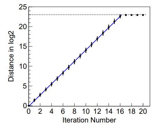
Figure 1. Separation of nearby trajectories for RANLUX.

Plotting the observed distance between two trajectories that start one bit apart, we find that the separation increases exponentially as shown in figure 1, but it requires about 15 iterations before the separation attains that expected for independent points, where we can say that the system attains the level of 2-mixing as defined above, and because of the ergodic hierarchy, this implies also 1-mixing and zero-mixing. That is a degree of randomness never before reached by any RNG.

But 2-mixing in RANLUX requires decimation of a factor of 15, which increases the time by about a factor eight, too slow for some applications. Since the slope of the exponential divergence of trajectories is equal to the logarithm of the largest eigenvalue (the Lyapunov exponent), speeding up the algorithm would require a matrix A with larger eigenvalues.

For those users who cannot afford the extra time taken for full decimation to 2-mixing, RANLUX already offered several luxury levels, which implement different amounts of decimation, according to the value of a parameter p defined such that after delivering 24 random numbers, would throw away p − 24 numbers before delivering the next 24, so that the highest standard luxury level corresponding to full 2-mixing would have p = 389.

MIXMAX

Even before RANLUX was published, George Savvidy in Erevan was working on a different approach to the same problem using the same theory of mixing. His method would be based on a matrix A which could be defined for any dimension N, having eigenvalues far from the unit circle and therefore large Lyapunov exponents, in order to reduce or possibly eliminate the need for decimation. For large N, the largest eigenvalue of the Savvidy matrix has a modulus approximately equal to N, much bigger than that of RANLUX.

But the problems of speed and period would prove exceptionally difficult, and it was only many years later that George’s son Konstantin Savvidy, also a theoretical physicist, was able to make use of the special structure of the matrix to perform the matrix-vector multiplication in time of order N, which made MIXMAX comparable in speed with the fastest RNG’s. He was also able to calculate the very long periods using finite (but large) Galois fields.

The implementation uses 64-bit integer arithmetic internally, and the user always gets standard double-precision floating-point numbers with 53- bit mantissas. The publication cited above gives the periods for 13 different values of the dimension N from 10 to 3150. All the periods are longer than 10165, so that is not a problem since it is physically impossible to generate that many numbers in the expected lifetime of the earth, even on quantum computers.

Unfortunately, the published paper does not mention decimation or the separation of nearby trajectories, so Lorenzo Moneta has calculated this separation as shown in figure 2 for 6 values of N from 10 to 1000.

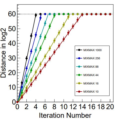
Figure 2. Separation of nearby trajectories for MIXMAX original.

It can be seen that all the separations increase exponentially and the required decimation to obtain 2-mixing decreases as N increases, as expected, so MIXMAX indeed behaves according to the theory and provided it is implemented with appropriate decimation, becomes the fastest RNG to guarantee 2-mixing.

However, the published algorithm and code do not implement decimation, so in order to obtain 2-mixing, it is necessary for the user to make a simple modification in the source code to accomplish this. CERN currently provides in ROOT a version of MIXMAX with N=256, appropriately modified to allow decimation.

Extended MIXMAX

In the search for a matrix with even larger eigenvalues, the developers of MIXMAX have introduced into the Savvidy matrix given above, a new parameter m in such a way that it does not interfere with the algorithm for fast multiplication and maintains the determinant =1. For very large values of m, the eigenvalues and periods of the new matrix are indeed spectacular, and promise very fast separation of nearby trajectories. However, as was the case for the original MIXMAX, the authors did not publish any results concerning the divergence of nearby trajectories for these generators. So we calculated this ourselves, and the results are shown in figure 3 for the three values of the parameters (N, s, m) which are recommended by the MIXMAX developers in a subsequent paper. It can be seen in figure 3 that the separation of trajectories does not increase exponentially as it should for a K-system.

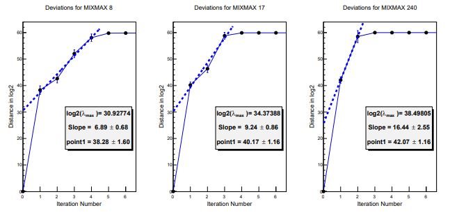
Figure 3. Separation of nearby trajectories for MIXMAX extended.

The problem is that for KA-mixing to occur, the discrete random numbers must be a sufficiently good approximation to continuous real numbers to follow the continuous trajectories of the mechanical system as it winds its way around the 256-dimensional torus, and the resolution required for this depends on the Lyapunov exponent of the system, the log of the largest eigenvalue. When this eigenvalue is too big, the trajectory of the continuous system winds around the torus so fast that the discrete points are not dense enough to follow the trajectory. Thus we see that when increasing the eigenvalues in order to reduce or eliminate decimation, we run into a kind of speed limit which requires a theory we don’t have.

RANLUX++

Recall that RANLUX was based on an algorithm by Marsaglia and Zaman which had exceptional speed and long period for generating single-precision floating-point numbers or 24-bit integers. When L¨uscher published RANLUX, it was already known that the Marsaglia-Zaman algorithm was exactly equivalent to a simple linear congruential generator (LCG) with an enormous multiplier, 576 bits long. This was used by L¨uscher to apply the spectral test to RANLUX, but otherwise was considered only of academic interest because computers of that time were not capable of multiplying such long integers in hardware. More recently however, this has become possible using new hardware instructions available on many computers but only in assembler code. In the paper cited above, Sibidanov shows how to use this to produce a version of RANLUX that looks like an LCG

Using his notation, one random integer (not a vector!) xi+1 is generated by x(i + 1) = a · x(i) mod m

To produce the same sequence as RANLUX, x is 24 bits long, the modulus m is 576 bits long, and the multiplier a is also 576 bits long. Implementing this formula directly requires multiplying two 576-bit integers, which using Sibidanov’s method can be done in a time comparable with the time required for native 64-bit integer multiplication.

But the more important gain comes when one applies decimation. Recall that decimation at level p in RANLUX means: deliver 24 numbers to the user, then throw away p - 24 numbers before delivering the next 24. In RANLUX++, it is implemented directly by x(i + p) = a p mod m · x(i) mod m where a^p mod m is a very long integer constant which can be pre-computed, so decimation in RANLUX++ is essentially done ”for free”, at least up to p=2048.

Moreover, when Sibidanov pre-computed the values of a^p mod m for different values of p corresponding to the standard luxury levels in RANLUX, as well as two new higher levels, p = 1024 and p = 2048, he got the surprising result shown below:

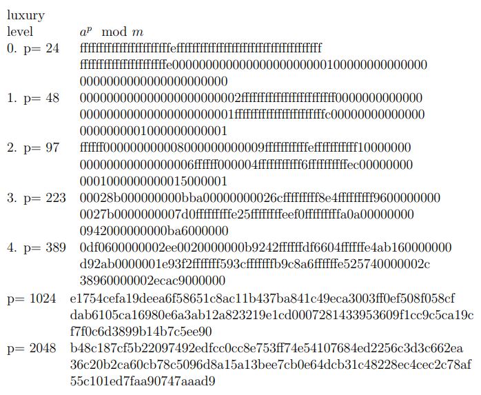
For values of p up to 389, the 144 hex digits are remarkably predictable, with exceptionally long sequences of 0’s and f’s, but this regularity decreases slowly with p until it is no longer obvious for p=1024 and 2048. Information Theory tells us that the information content of a message is proportional to the Shannon Entropy and is maximised when the digits are independent (no regularity). So what we are looking at is a set of long integer messages of increasing entropy, or information content. Since the information content is maximised when the digits are independent, let us test for independence using a statistical goodness-of-fit test called the runs test: For p= 1024 and 2048, the number of 2-runs and 3-runs (when 2 or 3 consecutive hex digits are the same), compared with number expected for 144 independent digits is:

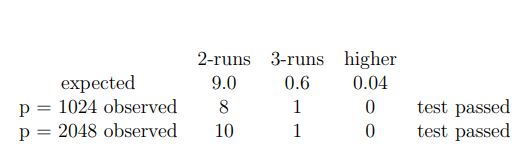
If the entropy of a p mod m is an indication of the degree of mixing, p = 389 is not enough, but p = 1024 is already fully mixing. Since decimation at level p = 2048 can be had ”for free” (in the same computer time as no decimation), RANLUX++ is much faster than the other algorithms for the higher levels of decimation

CONCLUSIONS

We now have three different algorithms capable of generating numbers that are random to the level of 2-mixing, and therefore also 1-mixing and zeromixing, provided the appropriate levels of decimation are applied. With these levels of decimation, the latest version of RANLUX single-precision is about as fast as MIXMAX (N=256, skip-5 decimation) double-precision. Where double precision is required, MIXMAX is about twice as fast. RANLUX++ is special because it requires assembler code which is of course not portable, but if portability is not a requirement, it is the fastest RNG to offer 2-mixing, and at the same time it can offer higher decimation with no penalty in speed.

We are currently investigating the possibility of attaining higher orders of mixing using higher levels of decimation, as suggested by the Shannon entropy content of the skipping factor a p mod m of RANLUX++. That probably implies finding a way of investigating the behaviour of a generator that is sensitive to the higher mixing and therefore the smaller eigenvalues (closer to one). We have therefore looked at RNG’s using the Savvidy matrix for which the ”magic integer” was purposely set to have an eigenvalue exactly on the unit circle so it would NOT be a K-system, and we observed that the random numbers nevertheless pass the best empirical tests of randomness (U01 Big Crush, for the experts), so we will need a to find a method which makes explicit use of the definition of 3-mixing for example. The separation of nearby trajectories is of course unable to detect the eigenvalue of modulus one, since it depends only on the largest eigenvalue.

References  

1. F. James and L. Moneta, Review of High-Quality Random Number Generators, https://link.springer.com/content/pdf/10.1007/s41781-019- 0034-3.pdf

2. M. L¨uscher, A Portable High-Quality Random Number Generator for Lattice Field Theory Simulations, Computer Physics Communications 79 (1994) 100

3. K.Savvidy, The MIXMAX random number generator, Comput.Phys.Commun. 196 (2015) 161-165. (http://dx.doi.org/10.1016/j.cpc.2015.06.003); arXiv:1404.5355

4. K. Savvidy and G. Savvidy, Spectrum and Entropy of C-systems. MIXMAX random number generator, Chaos Solitons Fractals 91 (2016) 33 [arXiv:1510.06274[math.DS]].

5. A. Sibidanov, A revision of the subtract-with-borrow random number generators, Comput. Phys. Comm. 221 (2017) 299-303